Cubes Tutorial 2 - Model and Mappings

In the first tutorial we talked about how to construct model programmatically and how to do basic aggregations.

In this tutorial we are going to learn:

• how to use model description file
• why and how to use logical to physical mappings

Data used are the same as in the first tutorial, IBRD Balance Sheet taken from The World Bank. However, for purpose of this tutorial, the file was little bit manually edited: the column “Line Item” is split into two: Subcategory and Line Item to provide two more levels to total of three levels of hierarchy.

Logical Model

The Cubes framework uses a logical model. Logical model describes the data from user’s or analyst’s perspective: data how they are being measured, aggregated and reported. Model creates an abstraction layer therefore making reports independent of physical structure of the data. More information can be found in the framework documentation

The model description file is a JSON file containing a dictionary:

{
    "dimensions": [  ...  ],
    "cubes": { ... }
}

First we define the dimensions. They might be shared by multiple cubes, therefore they belong to the model space. There are two dimensions: item and year in our dataset. The year dimension is flat, contains only one level and has no details. The dimension item has three levels: category, subcategory and line item. It looks like this:

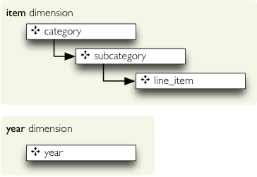
We define them as:

{
    "dimensions": [
        {"name":"item",
         "levels": ["category", "subcategory", "line_item"]
        },
        {"name":"year"}
    ],
    "cubes": {...}
}

The levels of our tutorial dimensions are simple, with no details. There is little bit of implicit construction going on behind the scenes of dimension initialization, but that will be described later. In short: default hierarchy is created and for each level single attribute is created with the same name as the level.

Next we define the cubes. The cube is in most cases specified by list of dimensions and measures:

{
    "dimensions": [...],
    "cubes": [
        {
            "name": "irbd_balance",
            "dimensions": ["item", "year"],
            "measures": ["amount"]
        }
    ]
}

And we are done: we have dimensions and a cube. Well, almost done: we have to tell the framework, which attributes are going to be used.

Attribute Naming

As mentioned before, cubes uses logical model to describe the data used in the reports. To assure consistency with dimension attribute naming, cubes uses sheme: dimension.attribute for non-flat dimensions. Why? Firstly, it decreases doubt to which dimension the attribute belongs. Secondly the item.category will always be item.category in the report, regardless of how the field will be named in the source and in which table the field exists.

Imagine a snowflake schema: fact table in the middle with references to multiple tables containing various dimension data. There might be a dimension spanning through multiple tables, like product category in one table, product subcategory in another table. We should not care about what table the attribute comes from, we should care only that the attribute is called category and belongs to a dimension product for example.

Another reason is, that in localized data, the analyst will use item.category_label and appropriate localized physical attribute will be used. Just to name few reasons.

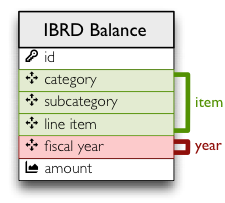
Knowing the naming scheme we have following cube attribute names:

• year (it is flat dimension)
• item.category
• item.subcategory
• item.line_item

Problem is, that the table does not have the columns with the names. That is what mapping is for: maps logical attributes in the model into physical attributes in the table.

Mapping

The source table looks like this:

We have to tell how the dimension attributes are mapped to the table columns. It is a simple dictionary where keys are dimension attribute names and values are physical table column names.

{
    ...
    "cubes": [
        {
            "name":"irbd_balance",
            ...
            "mappings": { "item.line_item": "line_item",
                          "item.subcategory": "subcategory",
                          "item.category": "category" }
        }
    ]
}

Note: The mapping values might be backend specific. They are physical table column names for the current implementation of the SQL backend.

Full model looks like this:

{
    "dimensions": [
        {"name":"item",
         "levels": ["category", "subcategory", "line_item"]
        },
        {"name":"year"}
    ],
    "cubes": [
        {
            "name":"irbd_balance",
            "dimensions": ["item", "year"],
            "measures": ["amount"],
            "mappings": { "item.line_item": "line_item",
                          "item.subcategory": "subcategory",
                          "item.category": "category" }
        }
        ]
    }
}

Example

Now we have the model, saved for example in the models/model_02.json. Let’s do some preparation:

Define table names and a view name to be used later. The view is going to be used as logical abstraction.

FACT_TABLE = "ft_irbd_balance"
FACT_VIEW = "vft_irbd_balance"

Load the data, as in the previous example, using the tutorial helper function (again, do not use that in production):

engine = sqlalchemy.create_engine('sqlite:///:memory:')
tutorial.create_table_from_csv(engine, 
                      "data/IBRD_Balance_Sheet__FY2010-t02.csv", 
                      table_name=FACT_TABLE, 
                      fields=[
                            ("category", "string"), 
                            ("subcategory", "string"), 
                            ("line_item", "string"),
                            ("year", "integer"), 
                            ("amount", "integer")],
                      create_id=True

                        )
connection = engine.connect()

The new data sheet is in the github repository.

Load the model, get the cube and specify where cube’s source data comes from:

workspace = cubes.Workspace()
workspace.import_model("models/model_02.json")
cube = workspace.cube("irbd_balance")
cube.fact = FACT_TABLE

We have to prepare the logical structures used by the browser. Currenlty provided is simple data denormalizer: creates one wide view with logical column names (optionally with localization). Following code initializes the denomralizer and creates a view for the cube:

dn = cubes.backends.sql.SQLDenormalizer(cube, connection)

dn.create_view(FACT_VIEW)

And from this point on, we can continue as usual:

browser = cubes.backends.sql.SQLBrowser(cube, connection, view_name = FACT_VIEW)

cell = cubes.Cell(cube)
result = browser.aggregate(cell)

print "Record count: %d" % result.summary["record_count"]
print "Total amount: %d" % result.summary["amount_sum"]

The tutorial sources can be found in the Cubes github repository. Requires current git clone.

Next: Drill-down through deep hierarchy.

If you have any questions, suggestions, comments, let me know.