How-to: hierarchies, levels and drilling-down

In this Cubes OLAP how-to we are going to learn:

• how to create a hierarchical dimension
• how to do drill-down through a hierarchy
• detailed level description

In the previous tutorial we learned how to use model descriptions in a JSON file and how to do physical to logical mappings.

Data used are similar as in the second tutorial, manually modified IBRD Balance Sheet taken from The World Bank. Difference between second tutorial and this one is added two columns: category code and sub-category code. They are simple letter codes for the categories and subcategories.

Hierarchy

Some dimensions can have multiple levels forming a hierarchy. For example dates have year, month, day; geography has country, region, city; product might have category, subcategory and the product.

Note: Cubes supports multiple hierarchies, for example for date you might have year-month-day or year-quarter-month-day. Most dimensions will have one hierarchy, thought.

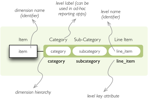
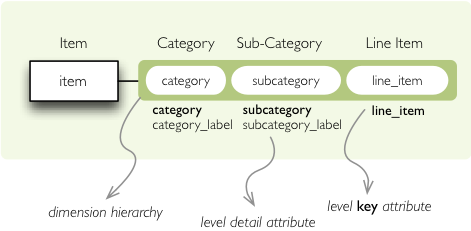
In our example we have the item dimension with three levels of hierarchy: category, subcategory and line item:

The levels are defined in the model:

"levels": [
    {
        "name":"category",
        "label":"Category",
        "attributes": ["category"]
    },
    {
        "name":"subcategory",
        "label":"Sub-category",
        "attributes": ["subcategory"]
    },
    {
        "name":"line_item",
        "label":"Line Item",
        "attributes": ["line_item"]
    }
]

You can see a slight difference between this model description and the previous one: we didn’t just specify level names and didn’t let cubes to fill-in the defaults. Here we used explicit description of each level. name is level identifier, label is human-readable label of the level that can be used in end-user applications and attributes is list of attributes that belong to the level. The first attribute, if not specified otherwise, is the key attribute of the level.

Other level description attributes are key and label_attribute. The key specifies attribute name which contains key for the level. Key is an id number, code or anything that uniquely identifies the dimension level. label_attribute is name of an attribute that contains human-readable value that can be displayed in user-interface elements such as tables or charts.

Preparation

In this how-to we are going to skip all off-topic code, such as data initialization. The full example can be found in the tutorial sources with suffix 03.

In short we need:

• data in a database
• logical model (see model_03.json) prepared with appropriate mappings
• denormalized view for aggregated browsing (for current simple SQL browser implementation)

Drill-down

Drill-down is an action that will provide more details about data. Drilling down through a dimension hierarchy will expand next level of the dimension. It can be compared to browsing through your directory structure.

We create a function that will recursively traverse a dimension hierarchy and will print-out aggregations (count of records in this example) at the actual browsed location.

Attributes

• cell - cube cell to drill-down
• dimension - dimension to be traversed through all levels
• path - current path of the dimension

Path is list of dimension points (keys) at each level. It is like file-system path.

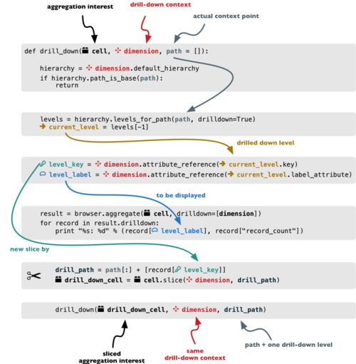
def drill_down(cell, dimension, path = []):

Get dimension’s default hierarchy. Cubes supports multiple hierarchies, for example for date you might have year-month-day or year-quarter-month-day. Most dimensions will have one hierarchy, thought.

    hierarchy = dimension.default_hierarchy

Base path is path to the most detailed element, to the leaf of a tree, to the fact. Can we go deeper in the hierarchy?

    if hierarchy.path_is_base(path):
        return

Get the next level in the hierarchy. levels_for_path returns list of levels according to provided path. When drilldown is set to True then one more level is returned.

    levels = hierarchy.levels_for_path(path,drilldown=True)
    current_level = levels[-1]

We need to know name of the level key attribute which contains a path component. If the model does not explicitly specify key attribute for the level, then first attribute will be used:

    level_key = dimension.attribute_reference(current_level.key)

For prettier display, we get name of attribute which contains label to be displayed for the current level. If there is no label attribute, then key attribute is used.

    level_label = dimension.attribute_reference(current_level.label_attribute)

We do the aggregation of the cell… Think of ls $CELL command in commandline, where $CELL is a directory name. In this function we can think of $CELL to be same as current working directory (pwd)

    result = browser.aggregate(cell, drilldown=[dimension])

    for record in result.drilldown:
        print "%s%s: %d" % (indent, record[level_label], record["record_count"])
        ...

And now the drill-down magic. First, construct new path by key attribute value appended to the current path:

        drill_path = path[:] + [record[level_key]]

Then get a new cell slice for current path:

        drill_down_cell = cell.slice(dimension, drill_path)

And do recursive drill-down:

        drill_down(drill_down_cell, dimension, drill_path)

The function looks like this:

Working function example 03 can be found in the tutorial sources.

Get the full cube (or any part of the cube you like):

cell = browser.full_cube()

And do the drill-down through the item dimension:

drill_down(cell, cube.dimension("item"))

The output should look like this:

a: 32
    da: 8
        Borrowings: 2
        Client operations: 2
        Investments: 2
        Other: 2
    dfb: 4
        Currencies subject to restriction: 2
        Unrestricted currencies: 2
    i: 2
        Trading: 2
    lo: 2
        Net loans outstanding: 2
    nn: 2
        Nonnegotiable, nonintrest-bearing demand obligations on account of subscribed capital: 2
    oa: 6
        Assets under retirement benefit plans: 2
        Miscellaneous: 2
        Premises and equipment (net): 2

Note that because we have changed our source data, we see level codes instead of level names. We will fix that later. Now focus on the drill-down.

See that nice hierarchy tree?

Now if you slice the cell through year 2010 and do the exact same drill-down:

    cell = cell.slice("year", [2010])
    drill_down(cell, cube.dimension("item"))

you will get similar tree, but only for year 2010 (obviously).

Level Labels and Details

Codes and ids are good for machines and programmers, they are short, might follow some scheme, easy to handle in scripts. Report users have no much use of them, as they look cryptic and have no meaning for the first sight.

Our source data contains two columns for category and for subcategory: column with code and column with label for user interfaces. Both columns belong to the same dimension and to the same level. The key column is used by the analytical system to refer to the dimension point and the label is just decoration.

Levels can have any number of detail attributes. The detail attributes have no analytical meaning and are just ignored during aggregations. If you want to do analysis based on an attribute, make it a separate dimension instead.

So now we fix our model by specifying detail attributes for the levels:

The model description is:

"levels": [
        {
            "name":"category",
            "label":"Category",
            "label_attribute": "category_label",
            "attributes": ["category", "category_label"]
        },
        {
            "name":"subcategory",
            "label":"Sub-category",
            "label_attribute": "subcategory_label",
            "attributes": ["subcategory", "subcategory_label"]
        },
        {
            "name":"line_item",
            "label":"Line Item",
            "attributes": ["line_item"]
        }
    ]
}

Note the label_attribute keys. They specify which attribute contains label to be displayed. Key attribute is by-default the first attribute in the list. If one wants to use some other attribute it can be specified in key_attribute.

Because we added two new attributes, we have to add mappings for them:

"mappings": { "item.line_item": "line_item",
              "item.subcategory": "subcategory",
              "item.subcategory_label": "subcategory_label",
              "item.category": "category",
              "item.category_label": "category_label" 
             }

In the example tutorial, which can be found in the Cubes sources under tutorial/ directory, change the model file from model/model_03.json to model/model_03-labels.json and run the code again. Or fix the file as specified above.

Now the result will be:

Assets: 32
    Derivative Assets: 8
        Borrowings: 2
        Client operations: 2
        Investments: 2
        Other: 2
    Due from Banks: 4
        Currencies subject to restriction: 2
        Unrestricted currencies: 2
    Investments: 2
        Trading: 2
    Loans Outstanding: 2
        Net loans outstanding: 2
    Nonnegotiable: 2
        Nonnegotiable, nonintrest-bearing demand obligations on account of subscribed capital: 2
    Other Assets: 6
        Assets under retirement benefit plans: 2
        Miscellaneous: 2
        Premises and equipment (net): 2

Implicit hierarchy

Try to remove the last level line_item from the model file and see what happens. Code still works, but displays only two levels. What does that mean? If metadata - logical model - is used properly in an application, then application can handle most of the model changes without any application modifications. That is, if you add new level or remove a level, there is no need to change your reporting application.

Summary

• hierarchies can have multiple levels
• a hierarchy level is identifier by a key attribute
• a hierarchy level can have multiple detail attributes and there is one special detail attribute: label attribute used for display in user interfaces

Next: slicing and dicing or slicer server, not sure yet.

If you have any questions, suggestions, comments, let me know.

Forking Forks with Higher Order Messaging

New way of constructing streams has been implemented which uses “higher order messaging”. What does that mean? Instead of constructing the stream from nodes and connections, you “call” functions that process your data. You pretend in your script that you work with data using functions:

...
main.csv_source("data.csv")
main.sample(1000)
main.aggregate(keys = ["year"])
main.formatted_printer()
...

Executing the functions as written in a script might be be very expensive from time and memory perspective. What is in fact happening is that instead of executing the data processing functions a stream network is being constructed.

Construction

Construction is being done by using forked branches. You create an empty forked branch by forking an empty stream:

from brewery.streams import *

stream = Stream()
main = stream.fork()
...

Now you have fork main. Each function call on main will append new processing node to the fork and the new node will be connected to the previous node of the fork.

Function names are based on node names in most of the cases. There might be custom function names for some nodes in the future, but now there is just simple rule:

1. decamelize node name: CSVSourceNode to csv source node
2. replace spaces with underscores: csv_source_node
3. remove ‘node’ suffix: csv_source

Arguments to the function are the same as arguments for node constructor. If you want to do more node configuration you can access current node with node attribute of the fork:

main.node.keys = ["country"]

Running

Run the stream as if it was constructed manually from nodes and connections:

stream.run()

Forking

So far you are able to construct single simple stream from a source to a target. There are plenty of situations where linear processing is not sufficient and you will need to have branches. To create another branch, you fork() a fork. For example, to attach data audit to the stream insert following code right after the node you want to audit:

# we are in main at node after which we want to have multiple branches

audit = main.fork()
audit.audit()
audit.value_threshold(...)
audit.formatted_printer(...)

# continue main.* branch here...

Example

Here is full example how to use forking with HOM in Brewery:

# Create the stream and empty fork
stream = Stream()
main = stream.fork()

# Start adding nodes by pretending that we are processing using functions
main.csv_source("data.csv", read_header = True, encoding = "utf-8")
main.coalesce_value_to_type()

# Create another fork for data audit:
audit = main.fork()
audit.audit(distinct_threshold = None)
audit.value_threshold(thresholds = [ ["null_record_ratio", 0.01] ],
                        bin_names = ("ok", "fail"))

audit.formatted_printer()
audit.node.header = u"field                            nulls     status   distinct\n" \
                         "------------------------------------------------------------"
audit.node.format = u"{field_name:7.2%} {null_record_ratio_bin:>10} {distinct_count:>10}"

# ...and we continue in main branch
main.database_table_target(url = "postgres://localhost/sandbox", 
                            table = "data",
                            create = True,
                            replace = True,
                            add_id_key = True)

# Run the stream and pretty-print the exception
try:
    stream.run()
except pipes.StreamRuntimeError, e:
    e.print_exception()

The constructed stream looks like this:

Brew data from Scraper Wiki

New subproject sprouted in Brewery: Opendata. The new package will contain wrappers for various open data services with APIs for structured data. First wrapper is for the Scraper Wiki. There are two new classes: ScraperWikiDataSource for plain data reading and ScraperWikiSourceNode for stream processing.

Example with ScraperWikiDataSource: Copy data from Scraper Wiki source into a local database. Table will be automatically created and replaced according to data structure in the source:

from brewery.opendata import *
from brewery.ds import *

src = ScraperWikiDataSource("seznam_insolvencnich_spravcu")
target = SQLDataTarget(url = "postgres://localhost/sandbox", table = "swiki_data",
                        create = True, replace = True)
src.initialize()
target.fields = src.fields
target.initialize()

for row in src.rows():
    target.append(row)

src.finalize()
target.finalize()

Another example using streams: simple completeness audit report of source data. Fail threshold is set to 10%.

The stream looks like this:

1. from scraper wiki feed data to data audit node
2. based on value threshold generate new textual field that will state whether the data passed or failed completeness test (there should be no more than 10% of empty values)
3. print formatted report

And the source code for the stream set-up is:

nodes = {
    "source": ScraperWikiSourceNode("seznam_insolvencnich_spravcu"),
    "audit": AuditNode(distinct_threshold = None),
    "threshold": ValueThresholdNode(),
    "print": FormattedPrinterNode(),
}

connections = [ 
                ("source", "audit"), 
                ("audit", "threshold"),
                ("threshold", "print")
                ]

nodes["print"].header = u"field                            nulls     status   distinct\n" \
                         "------------------------------------------------------------"
nodes["print"].format = u"{field_name:<30.30} {null_record_ratio: >7.2%} {null_record_ratio_bin:>10} {distinct_count:>10}"

nodes["threshold"].thresholds = [ ["null_record_ratio", 0.10] ]
nodes["threshold"].bin_names = ("ok", "fail")

stream = Stream(nodes, connections)

try:
    stream.run()
except StreamRuntimeError, e:
    e.print_exception()

Output:

field                            nulls     status   distinct
------------------------------------------------------------
cp_S                             0.00%         ok         84
cp_TP                           31.00%       fail         66
datumNarozeni                   18.00%       fail         83
denPozastaveni                 100.00%       fail          1
denVzniku                        0.00%         ok         91
denZaniku                      100.00%       fail          1
dne                             99.00%       fail          2
dobaPlatnosti                  100.00%       fail          1
...

nazev                           82.00%       fail         19
okres_S                          5.00%         ok         38
okres_TP                        38.00%       fail         35
...

In this example you can see how successful you scraper is or how complete the provided data are. This simple stream helps you to fine-tune your scraping method. 

Possible use, besides during development, would be to integrate the stream into automated process to get feedback on how complete your daily/monthly processing was.

In one of the following posts I will show you how to do “join” (in SQL sense) between datasets, for example how to enrich data from Scraper Wiki with details you have stored in a CSV or another scraper.