Star Browser, Part 3: Aggregations and Cell Details

Last time I was talking about joins and denormalisation in the Star Browser. This is the last part about the star browser where I will describe the aggregation and what has changed, compared to the old browser.

The Star Browser is new aggregation browser in for the Cubes – lightweight Python OLAP Framework. Next version v0.9 will be released next week.

Aggregation

sum is not the only aggregation. The new browser allows to have other aggregate functions as well, such as min, max.

You can specify the aggregations for each measure separately:

{
    "name": "amount",
    "aggregations": ["sum", "min", "max"]
}

The resulting aggregated attribute name will be constructed from the measure name and aggregation suffix, for example the mentioned amount will have three aggregates in the result: amount_sum, amount_min and amount_max.

Source code reference: see StarQueryBuilder.aggregations_for_measure

Aggregation Result

Result of aggregation is a structure containing: summary - summary for the aggregated cell, drilldown - drill down cells, if was desired, and total_cell_count - total cells in the drill down, regardless of pagination.

Cell Details

When we are browsing the cube, the cell provides current browsing context. For aggregations and selections to happen, only keys and some other internal attributes are necessary. Those can not be presented to the user though. For example we have geography path (country, region) as ['sk', 'ba'], however we want to display to the user Slovakia for the country and Bratislava for the region. We need to fetch those values from the data store. Cell details is basically a human readable description of the current cell.

For applications where it is possible to store state between aggregation calls, we can use values from previous aggregations or value listings. Problem is with web applications - sometimes it is not desirable or possible to store whole browsing context with all details. This is exact the situation where fetching cell details explicitly might come handy.

Note: The Original browser added cut information in the summary, which was ok when only point cuts were used. In other situations the result was undefined and mostly erroneous.

The cell details are now provided separately by method AggregationBrowser.cell_details(cell) which has Slicer HTTP equivalent /details or {"query":"detail", ...} in /report request. The result is a list of

For point cuts, the detail is a list of dictionaries for each level. For example our previously mentioned path ['sk', 'ba'] would have details described as:

[
    {
        "geography.country_code": "sk",
        "geography.country_name": "Slovakia",
        "geography.something_more": "..."
        "_key": "sk",
        "_label": "Slovakia"
    },
    {
        "geography.region_code": "ba",
        "geography.region_name": "Bratislava",
        "geography.something_even_more": "...",
        "_key": "ba",
        "_label": "Bratislava"
    }
]

You might have noticed the two redundant keys: _key and _label - those contain values of a level key attribute and level label attribute respectively. It is there to simplify the use of the details in presentation layer, such as templates. Take for example doing only one-dimensional browsing and compare presentation of "breadcrumbs":

labels = [detail["_label"] for detail in cut_details]

Which is equivalent to:

levels = dimension.hierarchy.levels()
labels = []
for i, detail in enumerate(cut_details):
    labels.append(detail[level[i].label_attribute.full_name()])

Note that this might change a bit: either full detail will be returned or just key and label, depending on an option argument (not yet decided).

Pre-aggregation

The Star Browser is being created with SQL pre-aggregation in mind. This is not possible in the old browser, as it is not flexible enough. It is planned to be integrated when all basic features are finished.

Proposed access from user's perspective will be through configuration options: use_preaggregation, preaggregation_prefix, preaggregation_schema and a method for cube pre-aggregation will be available through the slicer tool.

Summary

The new browser has better internal structure resulting in increased flexibility for future extensions. It fixes not so good architectural decisions of the old browser.

New and fixed features:

• direct star/snowflake schema browsing
• improved mappings - more transparent and understandable process
• ability to explicitly specify database schemas
• multiple aggregations

The new backend sources are here and the mapper is here.

To do

To be done in the near future:

• DDL generator for denormalized schema, corresponding logical schema and physical schema
• explicit list of attributes to be selected (instead of all)
• selection of aggregations per-request (now all specified in model are used)

Links

See also Cubes at github, Cubes Documentation, Mailing List and Submit issues. Also there is an IRC channel #databrewery on irc.freenode.net

Star Browser, Part 2: Joins and Denormalization

Last time I was talking about how logical attributes are mapped to the physical table columns in the Star Browser. Today I will describe how joins are formed and how denormalization is going to be used.

The Star Browser is new aggregation browser in for the Cubes – lightweight Python OLAP Framework.

Star, Snowflake, Master and Detail

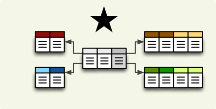
Star browser supports a star:

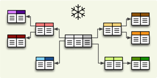
... and snowflake database schema:

The browser should know how to construct the star/snowflake and that is why you have to specify the joins of the schema. The join specification is very simple:

"joins" = [
    { "master": "fact_sales.product_id", "detail": "dim_product.id" }
]

Joins support only single-column keys, therefore you might have to create surrogate keys for your dimensions.

As in mappings, if you have specific needs for explicitly mentioning database schema or any other reason where table.column reference is not enough, you might write:

"joins" = [
    { 
        "master": "fact_sales.product_id",
        "detail": {
            "schema": "sales",
            "table": "dim_products",
            "column": "id"
        }
]

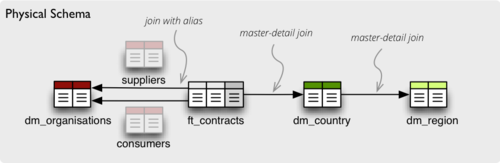
What if you need to join same table twice? For example, you have list of organizations and you want to use it as both: supplier and service consumer. It can be done by specifying alias in the joins:

"joins" = [
    {
        "master": "contracts.supplier_id", 
        "detail": "organisations.id",
        "alias": "suppliers"
    },
    {
        "master": "contracts.consumer_id", 
        "detail": "organisations.id",
        "alias": "consumers"
    }
]

In the mappings you refer to the table by alias specified in the joins, not by real table name:

"mappings": {
    "supplier.name": "suppliers.org_name",
    "consumer.name": "consumers.org_name"
}

Relevant Joins and Denormalization

The new mapper joins only tables that are relevant for given query. That is, if you are browsing by only one dimension, say product, then only product dimension table is joined.

Joins are slow, expensive and the denormalization can be helpful:

The old browser is based purely on the denormalized view. Despite having a performance gain, it has several disadvantages. From the join/performance perspective the major one is, that the denormalization is required and it is not possible to browse data in a database that was "read-only". This requirements was also one unnecessary step for beginners, which can be considered as usability problem.

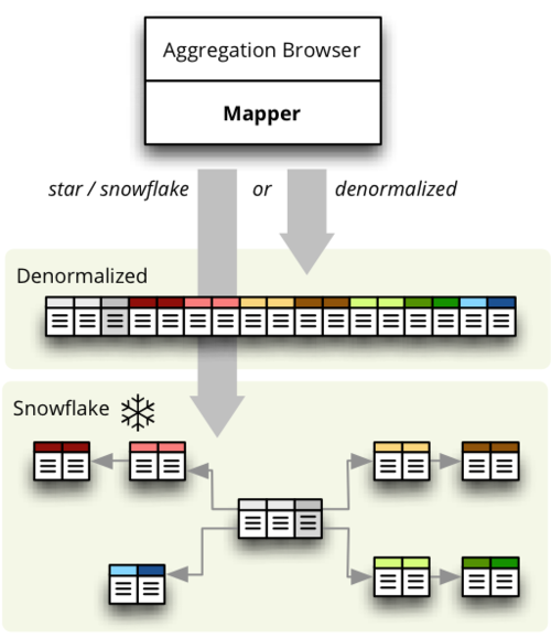
Current implementation of the Mapper and StarBrowser allows denormalization to be integrated in a way, that it might be used based on needs and situation:

It is not yet there and this is what needs to be done:

• function for denormalization - similar to the old one: will take cube and view name and will create denormalized view (or a table)
• make mapper accept the view and ignore joins

Goal is not just to slap denormalization in, but to make it a configurable alternative to default star browsing. From user's perspective, the workflow will be:

1. browse star/snowflake until need for denormalization arises
2. configure denormalization and create denormalized view
3. browse the denormalized view

The proposed options are: use_denormalization, denormalized_view_prefix, denormalized_view_schema.

The Star Browser is half-ready for the denormalization, just few changes are needed in the mapper and maybe query builder. These changes have to be compatible with another, not-yet-included feature: SQL pre-aggregation.

Conclusion

The new way of joining is very similar to the old one, but has much more cleaner code and is separated from mappings. Also it is more transparent. New feature is the ability to specify a database schema. Planned feature to be integrated is automatic join detection based on foreign keys.

In the next post (the last post in this series) about the new StarBrowser, I am going to explain aggregation improvements and changes.

Links

Relevant source code is this one (github).

See also Cubes at github, Cubes Documentation, Mailing List and Submit issues. Also there is an IRC channel #databrewery on irc.freenode.net

Star Browser, Part 1: Mappings

Star Browser is new aggregation browser in for the Cubes – lightweight Python OLAP Framework. I am going to talk briefly about current state and why new browser is needed. Then I will describe in more details the new browser: how mappings work, how tables are joined. At the end I will mention what will be added soon and what is planned in the future.

Originally I wanted to write one blog post about this, but it was too long, so I am going to split it into three:

• mappings (this one)
• joins and denormalization
• aggregations and new features

Why new browser?

Current denormalized browser is good, but not good enough. Firstly, it has grown into a spaghetti-like structure inside and adding new features is quite difficult. Secondly, it is not immediately clear what is going on inside and not only new users are getting into troubles. For example the mapping of logical to physical is not obvious; denormalization is forced to be used, which is good at the end, but is making OLAP newbies puzzled.

The new browser, called StarBrowser. is half-ready and will fix many of the old decisions with better ones.

Mapping

Cubes provides an analyst's view of dimensions and their attributes by hiding the physical representation of data. One of the most important parts of proper OLAP on top of the relational database is the mapping of physical attributes to logical.

First thing that was implemented in the new browser is proper mapping of logical attributes to physical table columns. For example, take a reference to an attribute name in a dimension product. What is the column of what table in which schema that contains the value of this dimension attribute?

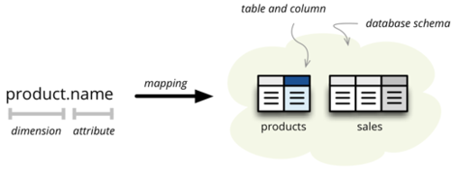
There are two ways how the mapping is being done: implicit and explicit. The simplest, straightforward and most customizable is the explicit way, where the actual column reference is provided in the model description:

"mappings": {
    "product.name": "dm_products.product_name"
}

If it is in different schema or any part of the reference contains a dot:

"mappings": {
    "product.name": {
            "schema": "sales",
            "table": "dm_products",
            "column": "product_name"
        }
}

Disadvantage of the explicit way is it's verbosity and the fact that developer has to write more metadata, obviously.

Both, explicit and implicit mappings have ability to specify default database schema (if you are using Oracle, PostgreSQL or any other DB which supports schemas).

The mapping process process is like this:

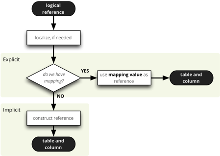
Implicit Mapping

With implicit mapping one can match a database schema with logical model and does not have to specify additional mapping metadata. Expected structure is star schema with one table per (denormalized) dimension.

Basic rules:

• fact table should have same name as represented cube
• dimension table should have same name as the represented dimension, for example: product (singular)
• references without dimension name in them are expected to be in the fact table, for example: amount, discount (see note below for simple flat dimensions)
• column name should have same name as dimension attribute: name, code, description
• if attribute is localized, then there should be one column per localization and should have locale suffix: description_en, description_sk, description_fr (see below for more information)

This means, that by default product.name is mapped to the table product and column name. Measure amount is mapped to the table sales and column amount

What about dimensions that have only one attribute, like one would not have a full date but just a year? In this case it is kept in the fact table without need of separate dimension table. The attribute is treated in by the same rule as measure and is referenced by simple year. This is applied to all dimensions that have only one attribute (representing key as well). This dimension is referred to as flat and without details.

Note for advanced users: this behavior can be disabled by setting simplify_dimension_references to False in the mapper. In that case you will have to have separate table for the dimension attribute and you will have to reference the attribute by full name. This might be useful when you know that your dimension will be more detailed.

Localization

Despite localization taking place first in the mapping process, we talk about it at the end, as it might be not so commonly used feature. From physical point of view, the data localization is very trivial and requires language denormalization - that means that each language has to have its own column for each attribute.

In the logical model, some of the attributes may contain list of locales that are provided for the attribute. For example product category can be in English, Slovak or German. It is specified in the model like this:

attributes = [{
    "name" = "category",
    "locales" = [en, sk, de],
}]

During the mapping process, localized logical reference is created first:

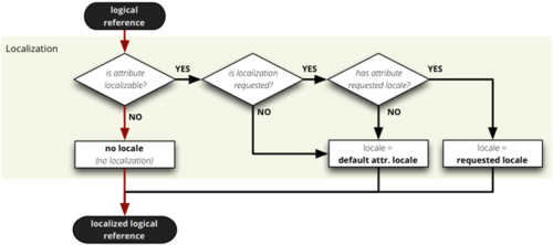
In short: if attribute is localizable and locale is requested, then locale suffix is added. If no such localization exists then default locale is used. Nothing happens to non-localizable attributes.

For such attribute, three columns should exist in the physical model. There are two ways how the columns should be named. They should have attribute name with locale suffix such as category_sk and category_en (underscore because it is more common in table column names), if implicit mapping is used. You can name the columns as you like, but you have to provide explicit mapping in the mapping dictionary. The key for the localized logical attribute should have .locale suffix, such as product.category.sk for Slovak version of category attribute of dimension product. Here the dot is used because dots separate logical reference parts.

Customization of the Implicit

The implicit mapping process has a little bit of customization as well:

• dimension table prefix: you can specify what prefix will be used for all dimension tables. For example if the prefix is dim_ and attribute is product.name then the table is going to be dim_product.
• fact table prefix: used for constructing fact table name from cube name. Example: having prefix ft_ all fact attributes of cube sales are going to be looked up in table ft_sales
• fact table name: one can explicitly specify fact table name for each cube separately

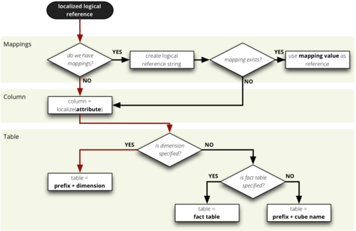
The Big Picture

Here is the whole mapping schema, after localization:

Links

The commented mapper source is here.

• github sources
• Documentation
• Mailing List
• Submit issues
• IRC channel #databrewery on irc.freenode.net

Cubes Backend Progress and Comparison

I've been working on a new SQL backend for cubes called StarBrowser. Besides new features and fixes, it is going to be more polished and maintainable.

Current Backend Comparison

In the following table you can see comparison of backends (or rather aggregation browsers). Current backend is sql.browser which reqiures denormalized table as a source. Future preferred backend will be sql.star.

Document link at Google Docs.

Star Browser state

More detailed description with schemas and description of what is happening behind will be published once the browser will be useable in most of the important features (that is, no sooner than drill-down is implemented). Here is a peek to the new browser features.

• separated attribute mapper - doing the logical-to-physical mapping. or in other words: knows what column in which table represents what dimension attribute or a measure
• more intelligent join building - uses only joins that are relevant to the retrieved attributes, does not join the whole star/snowflake if not necessary
• allows tables to be stored in different database schemas (previously everything had to be in one schema)

There is still some work to be done, including drill-down and ordering of results.

You can try limited feature set of the browser by using sql.star backend name. Do not expect much at this time, however if you find a bug, I would be glad if report it through github issues. The source is in the cubes/backends/sql/star.py and cubes/backends/sql/common.py (or here).

New and improved

Here is a list of features you can expect (not yet fully implemented, if at all started):

• more SQL aggregation types and way to specify what aggregations should be used by-default for each measure
• DDL schema generator for: denormalized table, logical model - star schema, physical model
• model tester - tests whether all attributes and joins are valid in the physical model

Also the new implementation of star browser will allow easier integration of pre-aggregated store (planned) and various other optimisations.

Data Streaming Basics in Brewery

How to build and run a data analysis stream? Why streams? I am going to talk about how to use brewery from command line and from Python scripts.

Brewery is a Python framework and a way of analysing and auditing data. Basic principle is flow of structured data through processing and analysing nodes. This architecture allows more transparent, understandable and maintainable data streaming process.

You might want to use brewery when you:

• want to learn more about data
• encounter unknown datasets and/or you do not know what you have in your datasets
• do not know exactly how to process your data and you want to play-around without getting lost
• want to create alternative analysis paths and compare them
• measure data quality and feed data quality results into the data processing process

There are many approaches and ways how to the data analysis. Brewery brings a certain workflow to the analyst:

1. examine data
2. prototype a stream (can use data sampling, not to overheat the machine)
3. see results and refine stream, create alternatives (at the same time)
4. repeat 3. until satisfied

Brewery makes the steps 2. and 3. easy - quick prototyping, alternative branching, comparison. Tries to keep the analysts workflow clean and understandable.

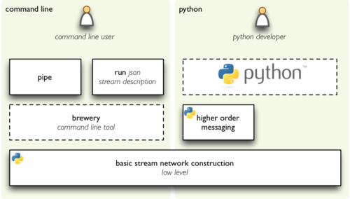
Building and Running a Stream

There are two ways to create a stream: programmatic in Python and command-line without Python knowledge requirement. Both ways have two alternatives: quick and simple, but with limited feature set. And the other is full-featured but is more verbose.

The two programmatic alternatives to create a stream are: basic construction and "HOM" or forking construction. The two command line ways to run a stream: run and pipe. We are now going to look closer at them.

Note regarding Zen of Python: this does not go against "There should be one – and preferably only one – obvious way to do it." There is only one way: the raw construction. The others are higher level ways or ways in different environments.

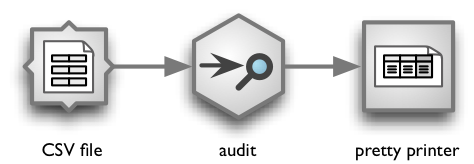
In our examples below we are going to demonstrate simple linear (no branching) stream that reads a CSV file, performs very basic audit and "pretty prints" out the result. The stream looks like this:

Command line

Brewery comes with a command line utility brewery which can run streams without needing to write a single line of python code. Again there are two ways of stream description: json-based and plain linear pipe.

The simple usage is with brewery pipe command:

brewery pipe csv_source resource=data.csv audit pretty_printer

The pipe command expects list of nodes and attribute=value pairs for node configuration. If there is no source pipe specified, CSV on standard input is used. If there is no target pipe, CSV on standard output is assumed:

cat data.csv | brewery pipe audit

The actual stream with implicit nodes is:

The json way is more verbose but is full-featured: you can create complex processing streams with many branches. stream.json:

    {
        "nodes": { 
            "source": { "type":"csv_source", "resource": "data.csv" },
            "audit":  { "type":"audit" },
            "target": { "type":"pretty_printer" }
        },
        "connections": [
            ["source", "audit"],
            ["audit", "target"]
        ]
    }

And run:

$ brewery run stream.json

To list all available nodes do:

$ brewery nodes

To get more information about a node, run brewery nodes:

$ brewery nodes string_strip

Note that data streaming from command line is more limited than the python way. You might not get access to nodes and node features that require python language, such as python storage type nodes or functions.

Higher order messaging

Preferred programming way of creating streams is through higher order messaging (HOM), which is, in this case, just fancy name for pretending doing something while in fact we are preparing the stream.

This way of creating a stream is more readable and maintainable. It is easier to insert nodes in the stream and create forks while not losing picture of the stream. Might be not suitable for very complex streams though. Here is an example:

    b = brewery.create_builder()
    b.csv_source("data.csv")
    b.audit()
    b.pretty_printer()

When this piece of code is executed, nothing actually happens to the data stream. The stream is just being prepared and you can run it anytime:

    b.stream.run()

What actually happens? The builder b is somehow empty object that accepts almost anything and then tries to find a node that corresponds to the method called. Node is instantiated, added to the stream and connected to the previous node.

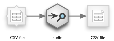
You can also create branched stream:

    b = brewery.create_builder()
    b.csv_source("data.csv")
    b.audit()

    f = b.fork()
    f.csv_target("audit.csv")

    b.pretty_printer()

Basic Construction

This is the lowest level way of creating the stream and allows full customisation and control of the stream. In the basic construction method the programmer prepares all node instance objects and connects them explicitly, node-by-node. Might be a too verbose, however it is to be used by applications that are constructing streams either using an user interface or from some stream descriptions. All other methods are using this one.

    from brewery import Stream
    from brewery.nodes import CSVSourceNode, AuditNode, PrettyPrinterNode

    stream = Stream()

    # Create pre-configured node instances
    src = CSVSourceNode("data.csv")
    stream.add(src)

    audit = AuditNode()
    stream.add(audit)

    printer = PrettyPrinterNode()
    stream.add(printer)

    # Connect nodes: source -> target
    stream.connect(src, audit)
    stream.connect(audit, printer)

    stream.run()

It is possible to pass nodes as dictionary and connections as list of tuples (source, target):

    stream = Stream(nodes, connections)

Future plans

What would be lovely to have in brewery?

Probing and data quality indicators – tools for simple data probing and easy way of creating data quality indicators. Will allow something like "test-driven-development" but for data. This is the next step.

Stream optimisation – merge multiple nodes into single processing unit before running the stream. Might be done in near future.

Backend-based nodes and related data transfer between backend nodes – For example, two SQL nodes might pass data through a database table instead of built-in data pipe or two numpy/scipy-based nodes might use numpy/scipy structure to pass data to avoid unnecessary streaming. Not very soon, but foreseeable future.

Stream compilation – compile a stream to an optimised script. Not too soon, but like to have that one.

Last, but not least: Currently there is little performance cost because of the nature of brewery implementation. This penalty will be explained in another blog post, however to make long story short, it has to do with threads, Python GIL and non-optimalized stream graph. There is no future prediction for this one, as it might be included step-by-step. Also some Python 3 features look promising, such as yield from in Python 3.3 (PEP 308).

Links

• Brewery at github
• Documentation and Node Reference
• Examples at github
• Google Group