Cubes - Python OLAP Framework Architecture

What is inside the Cubes Python OLAP Framework? Here is a brief overview of the core modules, their purpose and functionality.

The lightweight framework Cubes is composed of four public modules:

• model - Description of data (metadata): dimensions, hierarchies, attributes, labels, localizations.
• browser - Aggregation browsing, slicing-and-dicing, drill-down.
• backends - Actual aggregation implementation and utility functions.
• server - WSGI HTTP server for Cubes

Model

Logical model describes the data from user’s or analyst’s perspective: data how they are being measured, aggregated and reported. Model is independent of physical implementation of data. This physical independence makes it easier to focus on data instead on ways of how to get the data in understandable form.

Cubes model is described by:

• model object (doc)
• list of cubes
• dimensions of cubes (they are shared with all cubes within model) (doc) (doc)
• hierarchies (doc) and hierarchy levels (doc) of dimensions (such as category-subcategory, country-region-city)
• optional mappings from logical model to the physical model (doc)
• optional join specifications for star schemas, used by the SQL denormalizing backend (doc)

There is a utility function provided for loading the model from a JSON file: load_model.

The model module object are capable of being localized (see Model Localization for more information). The cubes provides localization at the metadata level (the model) and functionality to have localization at the data level.

See also: Model Documentation

Browser

Core of the Cubes analytics functionality is the aggregation browser. The browser module contains utility classes and functions for the browser to work.

The module components are:

• Cell – specification of the portion of the cube to be explored, sliced or drilled down. Each cell is specified by a set of cuts. A cell without any cuts represents whole cube.
• Cut – definition where the cell is going to be sliced through single dimension. There are three types of cuts: point, range and set.

The types of cuts:

• Point Cut – Defines one single point on a dimension where the cube is going to be sliced. The point might be at any level of hierarchy. The point is specified by "path". Examples of point cut: [2010] for year level of Date dimension, [2010,1,7] for full date point.
• Range Cut – Defines two points (dimension paths) on a sortable dimension between whose the cell is going to be sliced from cube.
• Set Cut – Defines list of multiple points (dimension paths) which are going to be included in the sliced cell.

Example of point cut effect:

The module provides couple utility functions:

• path_from_string - construct a dimension path (point) from a string
• string_from_path - get a string representation of a dimension path (point)
• string_from_cuts and cuts_from_string are for conversion between string and list of cuts. (Currently only list of point cuts are supported in the string representation)

The aggregation browser can:

• aggregate a cell (aggregate(cell))
• drill-down through multiple dimensions and aggregate (aggregate(cell, drilldown="date"))
• get all detailed facts within the cell (facts(cell))
• get single fact (fact(id))

There is convenience function report(cell, report) that can be implemented by backend in more efficient way to get multiple aggregation queries in single call.

More about aggregated browsing can be found in the Cubes documentation.

Backends

Actual aggregation is provided by the backends. The backend should implement aggregation browser interface.

Cubes comes with built-in ROLAP backend which uses SQL database through SQLAlchemy. The backend has two major components:

• aggregation browser that works on single denormalized view or a table
• SQL denormalizer helper class that converts star schema into a denormalized view or table (kind of materialisation).

There was an attempt to write a Mongo DB backend, but it does not work any more, it is included in the sources only as reminder, that there should be a mongo backend sometime in the future.

Anyone can write a backend. If you are interested, drop me a line.

Server

Cubes comes with Slicer - a WSGI HTTP OLAP server with API for most of the cubes framework functionality. The server is based on the Werkzeug framework.

Intended use of the slicer is basically as follows:

• application prepares the cell to be aggregated, drilled, listed... The cell might be whole cube.
• HTTP request is sent to the server
• the server uses appropriate aggregation browser backend (note that currently there is only one: SQL denormalized) to compute the request
• Slicer returns a JSON reply to the application

For more information, please refer to the Cubes Slicer server documentation.

One more thing...

There are plenty things to get improved, of course. Current focus is not on performance, but on achieving simple usability.

The Cubes sources can be found on Github: https://github.com/stiivi/cubes . There is also a IRC channel #databrewery on irc.freenode.net (I try to be there during late evening CET). Issues can be reported on the github project page.

If you have any questions, suggestions, recommendations, just let me know.

HackerNews Thread

Cubes 0.7.1 released

I am glad to announce new minor release of Cubes - Light Weight Python OLAP framework for multidimensional data aggregation and browsing. The news, changes and fixes are:

New Features

• New method: Dimension.attribute_reference: returns full reference to an attribute
• str(cut) will now return constructed string representation of a cut as it can be used by Slicer

Slicer server:

• added /locales to slicer
• added locales key in /model request
• added Access-Control-Allow-Origin for JS/jQuery

Changes

• Allow dimensions in cube to be a list, noy only a dictionary (internally it is ordered dictionary)
• Allow cubes in model to be a list, noy only a dictionary (internally it is ordered dictionary)

Slicer server:

• slicer does not require default cube to be specified: if no cube is in the request then try default from config or get first from model

Fixes

• Slicer not serves right localization regardless of what localization was used first after server was launched (changed model localization copy to be deepcopy (as it should be))
• Fixes some remnants that used old Cell.foo based browsing to Browser.foo(cell, ...) only browsing
• fixed model localization issues; once localized, original locale was not available
• Do not try to add locale if not specified. Fixes #11: https://github.com/Stiivi/cubes/issues/11

Tutorials

Added tutorials in tutorials/ with models in tutorials/models/ and data in tutorials/data/:

• Tutorial 1:
  • how to build a model programatically
  • how to create a model with flat dimensions
  • how to aggregate whole cube
  • how to drill-down and aggregate through a dimension
• Tutorial 2:
  • how to create and use a model file
  • mappings
• Tutorial 3:
  • how hierarhies work
  • drill-down through a hierarchy
• Tutorial 4 (not blogged about it yet):
  • how to launch slicer server

Links

• github sources: https://github.com/Stiivi/cubes
• Documentation: http://packages.python.org/cubes/
• Mailing List: http://groups.google.com/group/cubes-discuss
• Submit issues here: https://github.com/Stiivi/cubes/issues

If you have any questions, comments, requests, do not hesitate to ask.

How-to: hierarchies, levels and drilling-down

In this Cubes OLAP how-to we are going to learn:

• how to create a hierarchical dimension
• how to do drill-down through a hierarchy
• detailed level description

In the previous tutorial we learned how to use model descriptions in a JSON file and how to do physical to logical mappings.

Data used are similar as in the second tutorial, manually modified IBRD Balance Sheet taken from The World Bank. Difference between second tutorial and this one is added two columns: category code and sub-category code. They are simple letter codes for the categories and subcategories.

Hierarchy

Some dimensions can have multiple levels forming a hierarchy. For example dates have year, month, day; geography has country, region, city; product might have category, subcategory and the product.

Note: Cubes supports multiple hierarchies, for example for date you might have year-month-day or year-quarter-month-day. Most dimensions will have one hierarchy, thought.

In our example we have the item dimension with three levels of hierarchy: category, subcategory and line item:

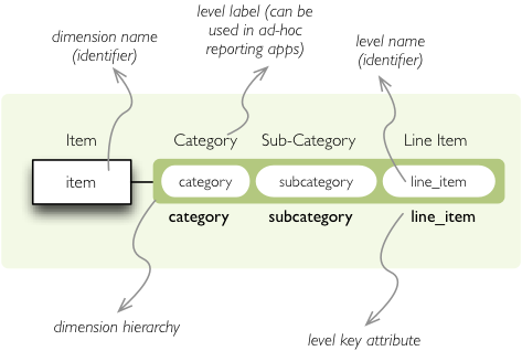
The levels are defined in the model:

"levels": [
    {
        "name":"category",
        "label":"Category",
        "attributes": ["category"]
    },
    {
        "name":"subcategory",
        "label":"Sub-category",
        "attributes": ["subcategory"]
    },
    {
        "name":"line_item",
        "label":"Line Item",
        "attributes": ["line_item"]
    }
]

You can see a slight difference between this model description and the previous one: we didn’t just specify level names and didn’t let cubes to fill-in the defaults. Here we used explicit description of each level. name is level identifier, label is human-readable label of the level that can be used in end-user applications and attributes is list of attributes that belong to the level. The first attribute, if not specified otherwise, is the key attribute of the level.

Other level description attributes are key and label_attribute. The key specifies attribute name which contains key for the level. Key is an id number, code or anything that uniquely identifies the dimension level. label_attribute is name of an attribute that contains human-readable value that can be displayed in user-interface elements such as tables or charts.

Preparation

In this how-to we are going to skip all off-topic code, such as data initialization. The full example can be found in the tutorial sources with suffix 03.

In short we need:

• data in a database
• logical model (see model_03.json) prepared with appropriate mappings
• denormalized view for aggregated browsing (for current simple SQL browser implementation)

Drill-down

Drill-down is an action that will provide more details about data. Drilling down through a dimension hierarchy will expand next level of the dimension. It can be compared to browsing through your directory structure.

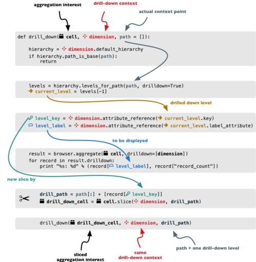
We create a function that will recursively traverse a dimension hierarchy and will print-out aggregations (count of records in this example) at the actual browsed location.

Attributes

• cell - cube cell to drill-down
• dimension - dimension to be traversed through all levels
• path - current path of the dimension

Path is list of dimension points (keys) at each level. It is like file-system path.

def drill_down(cell, dimension, path = []):

Get dimension’s default hierarchy. Cubes supports multiple hierarchies, for example for date you might have year-month-day or year-quarter-month-day. Most dimensions will have one hierarchy, thought.

    hierarchy = dimension.default_hierarchy

Base path is path to the most detailed element, to the leaf of a tree, to the fact. Can we go deeper in the hierarchy?

    if hierarchy.path_is_base(path):
        return

Get the next level in the hierarchy. levels_for_path returns list of levels according to provided path. When drilldown is set to True then one more level is returned.

    levels = hierarchy.levels_for_path(path,drilldown=True)
    current_level = levels[-1]

We need to know name of the level key attribute which contains a path component. If the model does not explicitly specify key attribute for the level, then first attribute will be used:

    level_key = dimension.attribute_reference(current_level.key)

For prettier display, we get name of attribute which contains label to be displayed for the current level. If there is no label attribute, then key attribute is used.

    level_label = dimension.attribute_reference(current_level.label_attribute)

We do the aggregation of the cell… Think of ls $CELL command in commandline, where $CELL is a directory name. In this function we can think of $CELL to be same as current working directory (pwd)

    result = browser.aggregate(cell, drilldown=[dimension])

    for record in result.drilldown:
        print "%s%s: %d" % (indent, record[level_label], record["record_count"])
        ...

And now the drill-down magic. First, construct new path by key attribute value appended to the current path:

        drill_path = path[:] + [record[level_key]]

Then get a new cell slice for current path:

        drill_down_cell = cell.slice(dimension, drill_path)

And do recursive drill-down:

        drill_down(drill_down_cell, dimension, drill_path)

The function looks like this:

Working function example 03 can be found in the tutorial sources.

Get the full cube (or any part of the cube you like):

cell = browser.full_cube()

And do the drill-down through the item dimension:

drill_down(cell, cube.dimension("item"))

The output should look like this:

a: 32
    da: 8
        Borrowings: 2
        Client operations: 2
        Investments: 2
        Other: 2
    dfb: 4
        Currencies subject to restriction: 2
        Unrestricted currencies: 2
    i: 2
        Trading: 2
    lo: 2
        Net loans outstanding: 2
    nn: 2
        Nonnegotiable, nonintrest-bearing demand obligations on account of subscribed capital: 2
    oa: 6
        Assets under retirement benefit plans: 2
        Miscellaneous: 2
        Premises and equipment (net): 2

Note that because we have changed our source data, we see level codes instead of level names. We will fix that later. Now focus on the drill-down.

See that nice hierarchy tree?

Now if you slice the cell through year 2010 and do the exact same drill-down:

    cell = cell.slice("year", [2010])
    drill_down(cell, cube.dimension("item"))

you will get similar tree, but only for year 2010 (obviously).

Level Labels and Details

Codes and ids are good for machines and programmers, they are short, might follow some scheme, easy to handle in scripts. Report users have no much use of them, as they look cryptic and have no meaning for the first sight.

Our source data contains two columns for category and for subcategory: column with code and column with label for user interfaces. Both columns belong to the same dimension and to the same level. The key column is used by the analytical system to refer to the dimension point and the label is just decoration.

Levels can have any number of detail attributes. The detail attributes have no analytical meaning and are just ignored during aggregations. If you want to do analysis based on an attribute, make it a separate dimension instead.

So now we fix our model by specifying detail attributes for the levels:

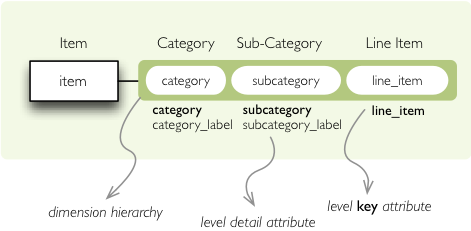
The model description is:

"levels": [
        {
            "name":"category",
            "label":"Category",
            "label_attribute": "category_label",
            "attributes": ["category", "category_label"]
        },
        {
            "name":"subcategory",
            "label":"Sub-category",
            "label_attribute": "subcategory_label",
            "attributes": ["subcategory", "subcategory_label"]
        },
        {
            "name":"line_item",
            "label":"Line Item",
            "attributes": ["line_item"]
        }
    ]
}

Note the label_attribute keys. They specify which attribute contains label to be displayed. Key attribute is by-default the first attribute in the list. If one wants to use some other attribute it can be specified in key_attribute.

Because we added two new attributes, we have to add mappings for them:

"mappings": { "item.line_item": "line_item",
              "item.subcategory": "subcategory",
              "item.subcategory_label": "subcategory_label",
              "item.category": "category",
              "item.category_label": "category_label" 
             }

In the example tutorial, which can be found in the Cubes sources under tutorial/ directory, change the model file from model/model_03.json to model/model_03-labels.json and run the code again. Or fix the file as specified above.

Now the result will be:

Assets: 32
    Derivative Assets: 8
        Borrowings: 2
        Client operations: 2
        Investments: 2
        Other: 2
    Due from Banks: 4
        Currencies subject to restriction: 2
        Unrestricted currencies: 2
    Investments: 2
        Trading: 2
    Loans Outstanding: 2
        Net loans outstanding: 2
    Nonnegotiable: 2
        Nonnegotiable, nonintrest-bearing demand obligations on account of subscribed capital: 2
    Other Assets: 6
        Assets under retirement benefit plans: 2
        Miscellaneous: 2
        Premises and equipment (net): 2

Implicit hierarchy

Try to remove the last level line_item from the model file and see what happens. Code still works, but displays only two levels. What does that mean? If metadata - logical model - is used properly in an application, then application can handle most of the model changes without any application modifications. That is, if you add new level or remove a level, there is no need to change your reporting application.

Summary

• hierarchies can have multiple levels
• a hierarchy level is identifier by a key attribute
• a hierarchy level can have multiple detail attributes and there is one special detail attribute: label attribute used for display in user interfaces

Next: slicing and dicing or slicer server, not sure yet.

If you have any questions, suggestions, comments, let me know.

Cubes Tutorial 2 - Model and Mappings

In the first tutorial we talked about how to construct model programmatically and how to do basic aggregations.

In this tutorial we are going to learn:

• how to use model description file
• why and how to use logical to physical mappings

Data used are the same as in the first tutorial, IBRD Balance Sheet taken from The World Bank. However, for purpose of this tutorial, the file was little bit manually edited: the column “Line Item” is split into two: Subcategory and Line Item to provide two more levels to total of three levels of hierarchy.

Logical Model

The Cubes framework uses a logical model. Logical model describes the data from user’s or analyst’s perspective: data how they are being measured, aggregated and reported. Model creates an abstraction layer therefore making reports independent of physical structure of the data. More information can be found in the framework documentation

The model description file is a JSON file containing a dictionary:

{
    "dimensions": [  ...  ],
    "cubes": { ... }
}

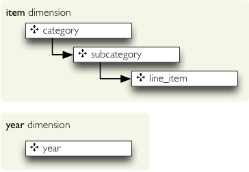
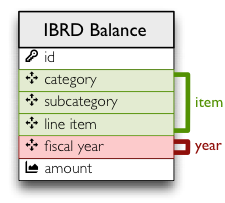
First we define the dimensions. They might be shared by multiple cubes, therefore they belong to the model space. There are two dimensions: item and year in our dataset. The year dimension is flat, contains only one level and has no details. The dimension item has three levels: category, subcategory and line item. It looks like this:

We define them as:

{
    "dimensions": [
        {"name":"item",
         "levels": ["category", "subcategory", "line_item"]
        },
        {"name":"year"}
    ],
    "cubes": {...}
}

The levels of our tutorial dimensions are simple, with no details. There is little bit of implicit construction going on behind the scenes of dimension initialization, but that will be described later. In short: default hierarchy is created and for each level single attribute is created with the same name as the level.

Next we define the cubes. The cube is in most cases specified by list of dimensions and measures:

{
    "dimensions": [...],
    "cubes": [
        {
            "name": "irbd_balance",
            "dimensions": ["item", "year"],
            "measures": ["amount"]
        }
    ]
}

And we are done: we have dimensions and a cube. Well, almost done: we have to tell the framework, which attributes are going to be used.

Attribute Naming

As mentioned before, cubes uses logical model to describe the data used in the reports. To assure consistency with dimension attribute naming, cubes uses sheme: dimension.attribute for non-flat dimensions. Why? Firstly, it decreases doubt to which dimension the attribute belongs. Secondly the item.category will always be item.category in the report, regardless of how the field will be named in the source and in which table the field exists.

Imagine a snowflake schema: fact table in the middle with references to multiple tables containing various dimension data. There might be a dimension spanning through multiple tables, like product category in one table, product subcategory in another table. We should not care about what table the attribute comes from, we should care only that the attribute is called category and belongs to a dimension product for example.

Another reason is, that in localized data, the analyst will use item.category_label and appropriate localized physical attribute will be used. Just to name few reasons.

Knowing the naming scheme we have following cube attribute names:

• year (it is flat dimension)
• item.category
• item.subcategory
• item.line_item

Problem is, that the table does not have the columns with the names. That is what mapping is for: maps logical attributes in the model into physical attributes in the table.

Mapping

The source table looks like this:

We have to tell how the dimension attributes are mapped to the table columns. It is a simple dictionary where keys are dimension attribute names and values are physical table column names.

{
    ...
    "cubes": [
        {
            "name":"irbd_balance",
            ...
            "mappings": { "item.line_item": "line_item",
                          "item.subcategory": "subcategory",
                          "item.category": "category" }
        }
    ]
}

Note: The mapping values might be backend specific. They are physical table column names for the current implementation of the SQL backend.

Full model looks like this:

{
    "dimensions": [
        {"name":"item",
         "levels": ["category", "subcategory", "line_item"]
        },
        {"name":"year"}
    ],
    "cubes": [
        {
            "name":"irbd_balance",
            "dimensions": ["item", "year"],
            "measures": ["amount"],
            "mappings": { "item.line_item": "line_item",
                          "item.subcategory": "subcategory",
                          "item.category": "category" }
        }
        ]
    }
}

Example

Now we have the model, saved for example in the models/model_02.json. Let’s do some preparation:

Define table names and a view name to be used later. The view is going to be used as logical abstraction.

FACT_TABLE = "ft_irbd_balance"
FACT_VIEW = "vft_irbd_balance"

Load the data, as in the previous example, using the tutorial helper function (again, do not use that in production):

engine = sqlalchemy.create_engine('sqlite:///:memory:')
tutorial.create_table_from_csv(engine, 
                      "data/IBRD_Balance_Sheet__FY2010-t02.csv", 
                      table_name=FACT_TABLE, 
                      fields=[
                            ("category", "string"), 
                            ("subcategory", "string"), 
                            ("line_item", "string"),
                            ("year", "integer"), 
                            ("amount", "integer")],
                      create_id=True

                        )
connection = engine.connect()

The new data sheet is in the github repository.

Load the model, get the cube and specify where cube’s source data comes from:

workspace = cubes.Workspace()
workspace.import_model("models/model_02.json")
cube = workspace.cube("irbd_balance")
cube.fact = FACT_TABLE

We have to prepare the logical structures used by the browser. Currenlty provided is simple data denormalizer: creates one wide view with logical column names (optionally with localization). Following code initializes the denomralizer and creates a view for the cube:

dn = cubes.backends.sql.SQLDenormalizer(cube, connection)

dn.create_view(FACT_VIEW)

And from this point on, we can continue as usual:

browser = cubes.backends.sql.SQLBrowser(cube, connection, view_name = FACT_VIEW)

cell = cubes.Cell(cube)
result = browser.aggregate(cell)

print "Record count: %d" % result.summary["record_count"]
print "Total amount: %d" % result.summary["amount_sum"]

The tutorial sources can be found in the Cubes github repository. Requires current git clone.

Next: Drill-down through deep hierarchy.

If you have any questions, suggestions, comments, let me know.

Cubes Tutorial 1 - Getting started

In this tutorial you are going to learn how to start with cubes. The example shows:

This tutorial is obsolete, please refer to the actual cubes documentation for more information.

• how to build a model programatically
• how to create a model with flat dimensions
• how to aggregate whole cube
• how to drill-down and aggregate through a dimension

The example data used are IBRD Balance Sheet taken from The World Bank

Create a tutorial directory and download the file:

curl -O https://raw.github.com/Stiivi/cubes/master/tutorial/data/IBRD_Balance_Sheet__FY2010.csv

Create a tutorial_01.py:

import sqlalchemy
import cubes
import cubes.tutorial.sql as tutorial

Cubes package contains tutorial helper methods. It is advised not to use them in production, they are provided just to simplify learner’s life.

Prepare the data using the tutorial helper methods:

engine = sqlalchemy.create_engine('sqlite:///:memory:')
tutorial.create_table_from_csv(engine, 
                      "IBRD_Balance_Sheet__FY2010.csv", 
                      table_name="irbd_balance", 
                      fields=[
                            ("category", "string"), 
                            ("line_item", "string"),
                            ("year", "integer"), 
                            ("amount", "integer")],
                      create_id=True    

                        )

Now, create a model:

model = cubes.Model()

Add dimensions to the model. Reason for having dimensions in a model is, that they might be shared by multiple cubes.

model.add_dimension(cubes.Dimension("category"))
model.add_dimension(cubes.Dimension("line_item"))
model.add_dimension(cubes.Dimension("year"))

Define a cube and specify already defined dimensions:

cube = cubes.Cube(name="irbd_balance", 
                  model=model,
                  dimensions=["category", "line_item", "year"],
                  measures=["amount"]
                  )

Create a browser and get a cell representing the whole cube (all data):

browser = cubes.backends.sql.SQLBrowser(cube, engine.connect(), view_name = "irbd_balance")

cell = browser.full_cube()

Compute the aggregate. Measure fields of aggregation result have aggregation suffix, currenlty only _sum. Also a total record count within the cell is included as record_count.

result = browser.aggregate(cell)

print "Record count: %d" % result.summary["record_count"]
print "Total amount: %d" % result.summary["amount_sum"]

Now try some drill-down by category:

print "Drill Down by Category"
result = browser.aggregate(cell, drilldown=["category"])

print "%-20s%10s%10s" % ("Category", "Count", "Total")
for record in result.drilldown:
    print "%-20s%10d%10d" % (record["category"], record["record_count"], record["amount_sum"])

Drill-dow by year:

print "Drill Down by Year:"
result = browser.aggregate(cell, drilldown=["year"])
print "%-20s%10s%10s" % ("Year", "Count", "Total")
for record in result.drilldown:
    print "%-20s%10d%10d" % (record["year"], record["record_count"], record["amount_sum"])

All tutorials with example data and models will be stored together with cubes sources under the tutorial/ directory.

Next: Model files and hierarchies.

If you have any questions, comments or suggestions, do not hesitate to ask.